Table of Contents
1 Malliavin calculus
1.1 Fractional Brownian motion
In the end of the 90’s, I worked on the stochastic analysis of the fractional Brownian motion decreusefond-1999-nil.
This is the very first example of a Gaussian process with tractable Gaussian covariance:
\[K_H(t,s):=\mathbf E[B^H(t)B^H(s)]=\frac12(s^{2H}+t^{2H}-|t-s|^{2H})\]
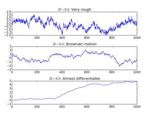
A basic code to simulate sample-paths of Brownian motion is the following. For a discretization \(t_i=iT/N,\ 1\le 0 \le N\), the random variables
\(( B^H(t_i), \ 1\le 0 \le N)\) form a Gaussian vector of correlation matrix:
\[\Gamma(i,j):=\operatorname{cov}( B^H(t_i),B^H(t_j))=K_H(t_i,t_j).\]
Thus, it can be simulated applying \(\Gamma^{1/2}\) to Gaussian unit vector. The square root of \(\Gamma\) trough the Cholesky decomposition.
from numpy import *
import numpy as np
import scipy
import scipy.linalg
import matplotlib.pyplot as plt


def noyau(H,x,y):
    return (x**(2*H)+y**(2*H)-np.abs(x-y)**(2*H))/2.

def covariance(nb_pts,H,horizon):
    t=(1+np.arange(nb_pts))*horizon/nb_pts/1.
    gam=np.empty([nb_pts,nb_pts])
    for i in np.arange(nb_pts):
        for j in np.arange(nb_pts-i):
            u=noyau(H,t[i],t[i+j])
            gam[i,i+j]=u
            gam[j+i,i]=u
    return np.array(scipy.linalg.cholesky(gam, lower=True))

def fbm(nb_pts,H,horizon):
    return np.dot(covariance(nb_pts,H,horizon),np.random.randn(nb_pts))

N=1000
horizon=10.


plt.subplot(3, 1, 1)
plt.plot(np.arange(N),fbm(N,0.3,horizon))
plt.title('$H=0.3$: Very rough')


plt.subplot(3, 1, 2)
plt.plot(np.arange(N),fbm(N,0.5,horizon))
plt.title('$H=0.5$: Brownian motion')

plt.subplot(3, 1, 3)
plt.plot(np.arange(N),fbm(N,0.9,horizon))
plt.title('$H=0.9$: Almost differentiable')


plt.tight_layout()
plt.show()
plt.savefig('fbm.pdf')
Actually, this was the very first paper to establish an Itô formula for this process. The sad reality is that this formula is absolutely useless as we do not have a nice stability result as for the ordinary Brownian motion:
\(\mathcal C^2\) transforms of semi-martingales are semi-martingales. It remains that it was a technical challenge to construct a stochastic integral with respect to this process, especially when its Hurst index is below \(1/3\). Concommitally, the rough paths theory initiated by Lyons Lyons1998 appeared and brillantly solved stochastic differential equations driven by a such a process. In fact, the theory is well developped only \(H>1/3\) whereas in DECREUSEFOND-2005 , the notion of stochastic integral for any \(H\), in any dimension, is defined and an Itô formula is established. However, no probabilistic method seems to exist so far to solve fBm driven SDEs for \(H<1/2\). The only purely random approach to SDE for \(H>1/2\) is given in Decreusefond-2013 via time reversal.
1.2 Independent random variables
Malliavin calculus is well defined for Gaussian and Poisson processes, be they in one dimension or higher. They share independent and stationary increments. Strangely enough, there does not seem to exist the counterpart for the simplest situation of independent random variables without the additional hypothesis of identical distribution. In this paper, we define a new discrete gradient close to some operators defined in Privault-2009 or in Boucheron-2013.
The two main applications of our framework are a chaos decomposition for the number of fixed points of a random permutations and a quantitative version of the Lyapounov central limit theorem for non identically distributed random variables.
Bibliography
- [decreusefond-1999-nil] Decreusefond & Üstünel, Stochastic analysis of fractional Brownian motion, Potential Analysis, 10(2), 177-214 (1999). link. doi.
- [Lyons1998] Lyons, Differential equations driven by rough signals., Revista Matemática Iberoamericana, 14(2), 215-310 (1998). link.
- [DECREUSEFOND-2005] Decreusefond, Stochastic integration with respect to Volterra processes, Annales de l’Institut Henri Poincare (B) Probability
and Statistics, 41(2), 123–149 (2005). link. doi. - [Decreusefond-2013] Decreusefond, Time Reversal of Volterra Processes Driven Stochastic Differential Equations, International Journal of Stochastic Analysis, 2013, 1–13 (2013). link. doi.
- [Privault-2009] Privault, Stochastic Analysis in Discrete and Continuous Settings, Lecture Notes in Mathematics, , (2009). link. doi.
- [Boucheron-2013] Boucheron, Lugosi, Massart & Pascal, Concentration Inequalities, , , (2013). link. doi.